最小化函数

minimize 函数

%pylab inline
set_printoptions(precision=3, suppress=True)

Populating the interactive namespace from numpy and matplotlib

已知斜抛运动的水平飞行距离公式：

$d = 2 \frac{v_0^2}{g} \sin(\theta) \cos (\theta)$

• $d$ 水平飞行距离
• $v_0$ 初速度大小
• $g$ 重力加速度
• $\theta$ 抛出角度

希望找到使 $d$ 最大的角度 $\theta$。

定义距离函数：

def dist(theta, v0):
    """calculate the distance travelled by a projectile launched
    at theta degrees with v0 (m/s) initial velocity.
    """
    g = 9.8
    theta_rad = pi * theta / 180
    return 2 * v0 ** 2 / g * sin(theta_rad) * cos(theta_rad)
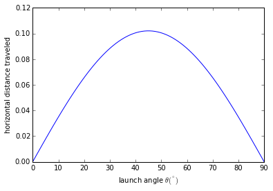
theta = linspace(0,90,90)
p = plot(theta, dist(theta, 1.))
xl = xlabel(r'launch angle $\theta (^{\circ})$')
yl = ylabel('horizontal distance traveled')

​

​

因为 Scipy 提供的是最小化方法，所以最大化距离就相当于最小化距离的负数：

def neg_dist(theta, v0):
    return -1 * dist(theta, v0)

导入 scipy.optimize.minimize：

from scipy.optimize import minimize
result = minimize(neg_dist, 40, args=(1,))
print "optimal angle = {:.1f} degrees".format(result.x[0])

optimal angle = 45.0 degrees

minimize 接受三个参数：第一个是要优化的函数，第二个是初始猜测值，第三个则是优化函数的附加参数，默认 minimize 将优化函数的第一个参数作为优化变量，所以第三个参数输入的附加参数从优化函数的第二个参数开始。

查看返回结果：

print result

   status: 0
  success: True
     njev: 18
     nfev: 54
 hess_inv: array([[ 8110.515]])
      fun: -0.10204079220645729
        x: array([ 45.02])
  message: 'Optimization terminated successfully.'
      jac: array([ 0.])

Rosenbrock 函数

Rosenbrock 函数是一个用来测试优化函数效果的一个非凸函数：

$f(x)=\sum\limits{i=1}^{N-1}{100\left(x{i+1}^2 - xi\right) ^2 + \left(1-x{i}\right)^2 }$

导入该函数：

from scipy.optimize import rosen
from mpl_toolkits.mplot3d import Axes3D

使用 N = 2 的 Rosenbrock 函数：

x, y = meshgrid(np.linspace(-2,2,25), np.linspace(-0.5,3.5,25))
z = rosen([x,y])

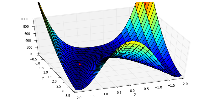
图像和最低点 (1,1)：

fig = figure(figsize=(12,5.5))
ax = fig.gca(projection="3d")
ax.azim = 70; ax.elev = 48
ax.set_xlabel("X"); ax.set_ylabel("Y")
ax.set_zlim((0,1000))
p = ax.plot_surface(x,y,z,rstride=1, cstride=1, cmap=cm.jet)
rosen_min = ax.plot([1],[1],[0],"ro")

​

​

传入初始值：

x0 = [1.3, 1.6, -0.5, -1.8, 0.8]
result = minimize(rosen, x0)
print result.x

[ 1.  1.  1.  1.  1.]

随机给定初始值：

x0 = np.random.randn(10)
result = minimize(rosen, x0)
print x0
print result.x

[ 0.815 -2.086  0.297  1.079 -0.528  0.461 -0.13  -0.715  0.734  0.621]
[-0.993  0.997  0.998  0.999  0.999  0.999  0.998  0.997  0.994  0.988]

对于 N > 3，函数的最小值为 $(x_1,x_2, ..., x_N) = (1,1,...,1)$，不过有一个局部极小值点 $(x_1,x_2, ..., x_N) = (-1,1,...,1)$，所以随机初始值如果选的不好的话，有可能返回的结果是局部极小值点：

优化方法

BFGS 算法

minimize 函数默认根据问题是否有界或者有约束，使用 'BFGS', 'L-BFGS-B', 'SLSQP' 中的一种。

可以查看帮助来得到更多的信息：

info(minimize)

 minimize(fun, x0, args=(), method=None, jac=None, hess=None, hessp=None,
          bounds=None, constraints=(), tol=None, callback=None, options=None)

Minimization of scalar function of one or more variables.

Parameters
----------
fun : callable
    Objective function.
x0 : ndarray
    Initial guess.
args : tuple, optional
    Extra arguments passed to the objective function and its
    derivatives (Jacobian, Hessian).
method : str or callable, optional
    Type of solver.  Should be one of

        - 'Nelder-Mead'
        - 'Powell'
        - 'CG'
        - 'BFGS'
        - 'Newton-CG'
        - 'Anneal (deprecated as of scipy version 0.14.0)'
        - 'L-BFGS-B'
        - 'TNC'
        - 'COBYLA'
        - 'SLSQP'
        - 'dogleg'
        - 'trust-ncg'
        - custom - a callable object (added in version 0.14.0)

    If not given, chosen to be one of `BFGS, L-BFGS-B, SLSQP`,
    depending if the problem has constraints or bounds.
jac : bool or callable, optional
    Jacobian (gradient) of objective function. Only for CG, BFGS,
    Newton-CG, L-BFGS-B, TNC, SLSQP, dogleg, trust-ncg.
    If jac is a Boolean and is True, fun is assumed to return the
    gradient along with the objective function. If False, the
    gradient will be estimated numerically.
    jac can also be a callable returning the gradient of the
    objective. In this case, it must accept the same arguments as fun.
hess, hessp : callable, optional
    Hessian (matrix of second-order derivatives) of objective function or
    Hessian of objective function times an arbitrary vector p.  Only for
    Newton-CG, dogleg, trust-ncg.
    Only one of hessp or hess needs to be given.  If hess is
    provided, then hessp will be ignored.  If neither hess nor
    hessp is provided, then the Hessian product will be approximated
    using finite differences on jac. hessp must compute the Hessian
    times an arbitrary vector.
bounds : sequence, optional
    Bounds for variables (only for L-BFGS-B, TNC and SLSQP).
    `(min, max) pairs for each element in x`, defining
    the bounds on that parameter. Use None for one of `min` or
    `max` when there is no bound in that direction.
constraints : dict or sequence of dict, optional
    Constraints definition (only for COBYLA and SLSQP).
    Each constraint is defined in a dictionary with fields:
        type : str
            Constraint type: 'eq' for equality, 'ineq' for inequality.
        fun : callable
            The function defining the constraint.
        jac : callable, optional
            The Jacobian of fun (only for SLSQP).
        args : sequence, optional
            Extra arguments to be passed to the function and Jacobian.
    Equality constraint means that the constraint function result is to
    be zero whereas inequality means that it is to be non-negative.
    Note that COBYLA only supports inequality constraints.
tol : float, optional
    Tolerance for termination. For detailed control, use solver-specific
    options.
options : dict, optional
    A dictionary of solver options. All methods accept the following
    generic options:
        maxiter : int
            Maximum number of iterations to perform.
        disp : bool
            Set to True to print convergence messages.
    For method-specific options, see :func:show_options().
callback : callable, optional
    Called after each iteration, as `callback(xk), where xk` is the
    current parameter vector.

Returns
-------
res : OptimizeResult
    The optimization result represented as a `OptimizeResult` object.
    Important attributes are: `x the solution array, success` a
    Boolean flag indicating if the optimizer exited successfully and
    `message` which describes the cause of the termination. See
    OptimizeResult for a description of other attributes.

​
​ See also
​ --------
​ minimize_scalar : Interface to minimization algorithms for scalar
​ univariate functions
​ show_options : Additional options accepted by the solvers
​

Notes
-----
This section describes the available solvers that can be selected by the
'method' parameter. The default method is *BFGS*.

**Unconstrained minimization**

Method *Nelder-Mead* uses the Simplex algorithm [1]_, [2]_. This
algorithm has been successful in many applications but other algorithms
using the first and/or second derivatives information might be preferred
for their better performances and robustness in general.

Method *Powell* is a modification of Powell's method [3]_, [4]_ which
is a conjugate direction method. It performs sequential one-dimensional
minimizations along each vector of the directions set (direc field in
options and info), which is updated at each iteration of the main
minimization loop. The function need not be differentiable, and no
derivatives are taken.

Method *CG* uses a nonlinear conjugate gradient algorithm by Polak and
Ribiere, a variant of the Fletcher-Reeves method described in [5]_ pp.
120-122. Only the first derivatives are used.

Method *BFGS* uses the quasi-Newton method of Broyden, Fletcher,
Goldfarb, and Shanno (BFGS) [5]_ pp. 136. It uses the first derivatives
only. BFGS has proven good performance even for non-smooth
optimizations. This method also returns an approximation of the Hessian
inverse, stored as hess_inv in the OptimizeResult object.

Method *Newton-CG* uses a Newton-CG algorithm [5]_ pp. 168 (also known
as the truncated Newton method). It uses a CG method to the compute the
search direction. See also *TNC* method for a box-constrained
minimization with a similar algorithm.

Method *Anneal* uses simulated annealing, which is a probabilistic
metaheuristic algorithm for global optimization. It uses no derivative
information from the function being optimized.

Method *dogleg* uses the dog-leg trust-region algorithm [5]_
for unconstrained minimization. This algorithm requires the gradient
and Hessian; furthermore the Hessian is required to be positive definite.

Method *trust-ncg* uses the Newton conjugate gradient trust-region
algorithm [5]_ for unconstrained minimization. This algorithm requires
the gradient and either the Hessian or a function that computes the
product of the Hessian with a given vector.

**Constrained minimization**

Method *L-BFGS-B* uses the L-BFGS-B algorithm [6]_, [7]_ for bound
constrained minimization.

Method *TNC* uses a truncated Newton algorithm [5]_, [8]_ to minimize a
function with variables subject to bounds. This algorithm uses
gradient information; it is also called Newton Conjugate-Gradient. It
differs from the *Newton-CG* method described above as it wraps a C
implementation and allows each variable to be given upper and lower
bounds.

Method *COBYLA* uses the Constrained Optimization BY Linear
Approximation (COBYLA) method [9]_, [10]_, [11]_. The algorithm is
based on linear approximations to the objective function and each
constraint. The method wraps a FORTRAN implementation of the algorithm.

Method *SLSQP* uses Sequential Least SQuares Programming to minimize a
function of several variables with any combination of bounds, equality
and inequality constraints. The method wraps the SLSQP Optimization
subroutine originally implemented by Dieter Kraft [12]_. Note that the
wrapper handles infinite values in bounds by converting them into large
floating values.

**Custom minimizers**

It may be useful to pass a custom minimization method, for example
when using a frontend to this method such as scipy.optimize.basinhopping
or a different library.  You can simply pass a callable as the `method`
parameter.

The callable is called as `method(fun, x0, args, **kwargs, **options)`
where `kwargs corresponds to any other parameters passed to minimize`
(such as callback, hess, etc.), except the options dict, which has
its contents also passed as method parameters pair by pair.  Also, if
jac has been passed as a bool type, jac and fun are mangled so that
fun returns just the function values and jac is converted to a function
returning the Jacobian.  The method shall return an `OptimizeResult`
object.

The provided method callable must be able to accept (and possibly ignore)
arbitrary parameters; the set of parameters accepted by minimize may
expand in future versions and then these parameters will be passed to
the method.  You can find an example in the scipy.optimize tutorial.

.. versionadded:: 0.11.0

References
----------
.. [1] Nelder, J A, and R Mead. 1965. A Simplex Method for Function
    Minimization. The Computer Journal 7: 308-13.
.. [2] Wright M H. 1996. Direct search methods: Once scorned, now
    respectable, in Numerical Analysis 1995: Proceedings of the 1995
    Dundee Biennial Conference in Numerical Analysis (Eds. D F
    Griffiths and G A Watson). Addison Wesley Longman, Harlow, UK.
    191-208.
.. [3] Powell, M J D. 1964. An efficient method for finding the minimum of
   a function of several variables without calculating derivatives. The
   Computer Journal 7: 155-162.
.. [4] Press W, S A Teukolsky, W T Vetterling and B P Flannery.
   Numerical Recipes (any edition), Cambridge University Press.
.. [5] Nocedal, J, and S J Wright. 2006. Numerical Optimization.
   Springer New York.
.. [6] Byrd, R H and P Lu and J. Nocedal. 1995. A Limited Memory
   Algorithm for Bound Constrained Optimization. SIAM Journal on
   Scientific and Statistical Computing 16 (5): 1190-1208.
.. [7] Zhu, C and R H Byrd and J Nocedal. 1997. L-BFGS-B: Algorithm
   778: L-BFGS-B, FORTRAN routines for large scale bound constrained
   optimization. ACM Transactions on Mathematical Software 23 (4):
   550-560.
.. [8] Nash, S G. Newton-Type Minimization Via the Lanczos Method.
   1984. SIAM Journal of Numerical Analysis 21: 770-778.
.. [9] Powell, M J D. A direct search optimization method that models
   the objective and constraint functions by linear interpolation.
   1994. Advances in Optimization and Numerical Analysis, eds. S. Gomez
   and J-P Hennart, Kluwer Academic (Dordrecht), 51-67.
.. [10] Powell M J D. Direct search algorithms for optimization
   calculations. 1998. Acta Numerica 7: 287-336.
.. [11] Powell M J D. A view of algorithms for optimization without
   derivatives. 2007.Cambridge University Technical Report DAMTP
   2007/NA03
.. [12] Kraft, D. A software package for sequential quadratic
   programming. 1988. Tech. Rep. DFVLR-FB 88-28, DLR German Aerospace
   Center -- Institute for Flight Mechanics, Koln, Germany.

Examples
--------
Let us consider the problem of minimizing the Rosenbrock function. This
function (and its respective derivatives) is implemented in rosen
(resp. rosen_der, rosen_hess) in the scipy.optimize.

>>> from scipy.optimize import minimize, rosen, rosen_der

A simple application of the *Nelder-Mead* method is:

>>> x0 = [1.3, 0.7, 0.8, 1.9, 1.2]
>>> res = minimize(rosen, x0, method='Nelder-Mead')
>>> res.x
[ 1.  1.  1.  1.  1.]

Now using the *BFGS* algorithm, using the first derivative and a few
options:

>>> res = minimize(rosen, x0, method='BFGS', jac=rosen_der,
...                options={'gtol': 1e-6, 'disp': True})
Optimization terminated successfully.
         Current function value: 0.000000
         Iterations: 52
         Function evaluations: 64
         Gradient evaluations: 64
>>> res.x
[ 1.  1.  1.  1.  1.]
>>> print res.message
Optimization terminated successfully.
>>> res.hess
[[ 0.00749589  0.01255155  0.02396251  0.04750988  0.09495377]
 [ 0.01255155  0.02510441  0.04794055  0.09502834  0.18996269]
 [ 0.02396251  0.04794055  0.09631614  0.19092151  0.38165151]
 [ 0.04750988  0.09502834  0.19092151  0.38341252  0.7664427 ]
 [ 0.09495377  0.18996269  0.38165151  0.7664427   1.53713523]]

​
​ Next, consider a minimization problem with several constraints (namely
​ Example 16.4 from [5]_). The objective function is:
​

>>> fun = lambda x: (x[0] - 1)**2 + (x[1] - 2.5)**2

There are three constraints defined as:

>>> cons = ({'type': 'ineq', 'fun': lambda x:  x[0] - 2 * x[1] + 2},
...         {'type': 'ineq', 'fun': lambda x: -x[0] - 2 * x[1] + 6},
...         {'type': 'ineq', 'fun': lambda x: -x[0] + 2 * x[1] + 2})

And variables must be positive, hence the following bounds:

>>> bnds = ((0, None), (0, None))

The optimization problem is solved using the SLSQP method as:

>>> res = minimize(fun, (2, 0), method='SLSQP', bounds=bnds,
...                constraints=cons)

It should converge to the theoretical solution (1.4 ,1.7).

默认没有约束时，使用的是 BFGS 方法。

利用 callback 参数查看迭代的历史：

x0 = [-1.5, 4.5]
xi = [x0]
result = minimize(rosen, x0, callback=xi.append)
xi = np.asarray(xi)
print xi.shape
print result.x
print "in {} function evaluations.".format(result.nfev)

(37L, 2L)
[ 1.  1.]
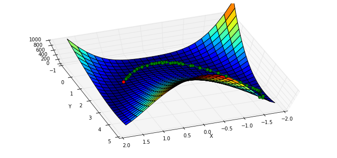
in 200 function evaluations.

绘图显示轨迹：

x, y = meshgrid(np.linspace(-2.3,1.75,25), np.linspace(-0.5,4.5,25))
z = rosen([x,y])
fig = figure(figsize=(12,5.5))
ax = fig.gca(projection="3d"); ax.azim = 70; ax.elev = 75
ax.set_xlabel("X"); ax.set_ylabel("Y"); ax.set_zlim((0,1000))
p = ax.plot_surface(x,y,z,rstride=1, cstride=1, cmap=cm.jet)
intermed = ax.plot(xi[:,0], xi[:,1], rosen(xi.T), "g-o")
rosen_min = ax.plot([1],[1],[0],"ro")

​

​

BFGS 需要计算函数的 Jacobian 矩阵：

给定 $\left[y_1,y_2,y_3\right] = f(x_0, x_1, x_2)$

$$J=\left[ \begin{matrix} \frac{\partial y_1}{\partial x_0} & \frac{\partial y_1}{\partial x_1} & \frac{\partial y_1}{\partial x_2} \\ \frac{\partial y_2}{\partial x_0} & \frac{\partial y_2}{\partial x_1} & \frac{\partial y_2}{\partial x_2} \\ \frac{\partial y_3}{\partial x_0} & \frac{\partial y_3}{\partial x_1} & \frac{\partial y_3}{\partial x_2} \end{matrix} \right]$$

在我们的例子中

$$J= \left[ \begin{matrix}\frac{\partial rosen}{\partial x_0} & \frac{\partial rosen}{\partial x_1} \end{matrix} \right] $$

导入 rosen 函数的 Jacobian 函数 rosen_der：

from scipy.optimize import rosen_der

此时，我们将 Jacobian 矩阵作为参数传入：

xi = [x0]
result = minimize(rosen, x0, jac=rosen_der, callback=xi.append)
xi = np.asarray(xi)
print xi.shape
print "in {} function evaluations and {} jacobian evaluations.".format(result.nfev, result.njev)

(38L, 2L)
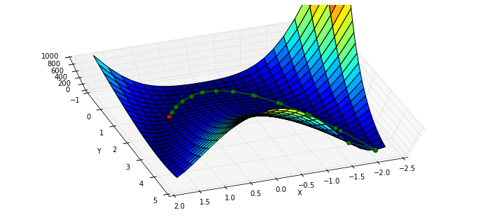
in 49 function evaluations and 49 jacobian evaluations.

可以看到，函数计算的开销大约减少了一半，迭代路径与上面的基本吻合：

x, y = meshgrid(np.linspace(-2.3,1.75,25), np.linspace(-0.5,4.5,25))
z = rosen([x,y])
fig = figure(figsize=(12,5.5))
ax = fig.gca(projection="3d"); ax.azim = 70; ax.elev = 75
ax.set_xlabel("X"); ax.set_ylabel("Y"); ax.set_zlim((0,1000))
p = ax.plot_surface(x,y,z,rstride=1, cstride=1, cmap=cm.jet)
intermed = ax.plot(xi[:,0], xi[:,1], rosen(xi.T), "g-o")
rosen_min = ax.plot([1],[1],[0],"ro")

​

​

Nelder-Mead Simplex 算法

改变 minimize 使用的算法，使用 Nelder–Mead 单纯形算法：

xi = [x0]
result = minimize(rosen, x0, method="nelder-mead", callback = xi.append)
xi = np.asarray(xi)
print xi.shape
print "Solved the Nelder-Mead Simplex method with {} function evaluations.".format(result.nfev)

(120L, 2L)
Solved the Nelder-Mead Simplex method with 226 function evaluations.

x, y = meshgrid(np.linspace(-1.9,1.75,25), np.linspace(-0.5,4.5,25))
z = rosen([x,y])
fig = figure(figsize=(12,5.5))
ax = fig.gca(projection="3d"); ax.azim = 70; ax.elev = 75
ax.set_xlabel("X"); ax.set_ylabel("Y"); ax.set_zlim((0,1000))
p = ax.plot_surface(x,y,z,rstride=1, cstride=1, cmap=cm.jet)
intermed = ax.plot(xi[:,0], xi[:,1], rosen(xi.T), "g-o")
rosen_min = ax.plot([1],[1],[0],"ro")

​

​

Powell 算法

使用 Powell 算法

xi = [x0]
result = minimize(rosen, x0, method="powell", callback=xi.append)
xi = np.asarray(xi)
print xi.shape
print "Solved Powell's method with {} function evaluations.".format(result.nfev)

(31L, 2L)
Solved Powell's method with 855 function evaluations.

x, y = meshgrid(np.linspace(-2.3,1.75,25), np.linspace(-0.5,4.5,25))
z = rosen([x,y])
fig = figure(figsize=(12,5.5))
ax = fig.gca(projection="3d"); ax.azim = 70; ax.elev = 75
ax.set_xlabel("X"); ax.set_ylabel("Y"); ax.set_zlim((0,1000))
p = ax.plot_surface(x,y,z,rstride=1, cstride=1, cmap=cm.jet)
intermed = ax.plot(xi[:,0], xi[:,1], rosen(xi.T), "g-o")
rosen_min = ax.plot([1],[1],[0],"ro")

​

​