积分

符号积分

积分与求导的关系：

$$\frac{d}{dx} F(x) = f(x)
\Rightarrow F(x) = \int f(x) dx$$

符号运算可以用 sympy 模块完成。

先导入 init_printing 模块方便其显示：

from sympy import init_printing
init_printing()

from sympy import symbols, integrate
import sympy

产生 x 和 y 两个符号变量，并进行运算：

x, y = symbols('x y')
sympy.sqrt(x ** 2 + y ** 2)

$$\sqrt{x^{2} + y^{2}}$$

对于生成的符号变量 z，我们将其中的 x 利用 subs 方法替换为 3：

z = sympy.sqrt(x ** 2 + y ** 2)
z.subs(x, 3)

$$\sqrt{y^{2} + 9}$$

再替换 y：

z.subs(x, 3).subs(y, 4)

$$5$$

还可以从 sympy.abc 中导入现成的符号变量：

from sympy.abc import theta
y = sympy.sin(theta) ** 2
y

$$\sin^{2}{\left (\theta \right )}$$

对 y 进行积分：

Y = integrate(y)
Y

$$\frac{\theta}{2} - \frac{1}{2} \sin{\left (\theta \right )} \cos{\left (\theta \right )}$$

计算 $Y(\pi) - Y(0)$：

import numpy as np
np.set_printoptions(precision=3)

Y.subs(theta, np.pi) - Y.subs(theta, 0)

$$1.5707963267949$$

计算 $\int_0^\pi y d\theta$ ：

integrate(y, (theta, 0, sympy.pi))

$$\frac{\pi}{2}$$

显示的是字符表达式，查看具体数值可以使用 evalf() 方法，或者传入 numpy.pi，而不是 sympy.pi ：

integrate(y, (theta, 0, sympy.pi)).evalf()

$$1.5707963267949$$

integrate(y, (theta, 0, np.pi))

$$1.5707963267949$$

根据牛顿莱布尼兹公式，这两个数值应该相等。

产生不定积分对象：

Y_indef = sympy.Integral(y)
Y_indef

$$\int \sin^{2}{\left (\theta \right )}\, d\theta$$

print type(Y_indef)

定积分：

Y_def = sympy.Integral(y, (theta, 0, sympy.pi))
Y_def

$$\int_{0}^{\pi} \sin^{2}{\left (\theta \right )}\, d\theta$$

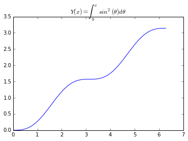
产生函数 $Y(x) = \int_0^x sin^2(\theta) d\theta$，并将其向量化：

Y_raw = lambda x: integrate(y, (theta, 0, x))
Y = np.vectorize(Y_raw)

%matplotlib inline
import matplotlib.pyplot as plt

x = np.linspace(0, 2 * np.pi)
p = plt.plot(x, Y(x))
t = plt.title(r'$Y(x) = \int_0^x sin^2(\theta) d\theta$')

​

​

数值积分

数值积分：

$$F(x) = \lim{n \rightarrow \infty} \sum{i=0}^{n-1} f(xi)(x{i+1}-xi)
\Rightarrow F(x) = \int{x_0}^{x_n} f(x) dx$$

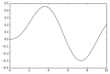
导入贝塞尔函数：

from scipy.special import jv

def f(x):
    return jv(2.5, x)

x = np.linspace(0, 10)
p = plt.plot(x, f(x), 'k-')

​

​

quad 函数

Quadrature 积分的原理参见：

http://en.wikipedia.org/wiki/Numerical_integration#Quadrature_rules_based_on_interpolating_functions

quad 返回一个 (积分值，误差) 组成的元组：

from scipy.integrate import quad
interval = [0, 6.5]
value, max_err = quad(f, *interval)

积分值：

print value

1.28474297234

最大误差：

print max_err

2.34181853668e-09

积分区间图示，蓝色为正，红色为负：

print "integral = {:.9f}".format(value)
print "upper bound on error: {:.2e}".format(max_err)
x = np.linspace(0, 10, 100)
p = plt.plot(x, f(x), 'k-')
x = np.linspace(0, 6.5, 45)
p = plt.fill_between(x, f(x), where=f(x)>0, color="blue")
p = plt.fill_between(x, f(x), where=f(x)<0, color="red", interpolate=True)

integral = 1.284742972
upper bound on error: 2.34e-09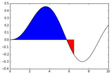

积分到无穷

from numpy import inf
interval = [0., inf]

def g(x):
    return np.exp(-x ** 1/2)

value, max_err = quad(g, *interval)
x = np.linspace(0, 10, 50)
fig = plt.figure(figsize=(10,3))
p = plt.plot(x, g(x), 'k-')
p = plt.fill_between(x, g(x))
plt.annotate(r"$\int_0^{\infty}e^{-x^1/2}dx = $" + "{}".format(value), (4, 0.6),
         fontsize=16)
print "upper bound on error: {:.1e}".format(max_err)

upper bound on error: 7.2e-11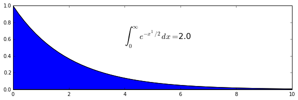

双重积分

假设我们要进行如下的积分：

$$ I_n = \int \limits_0^{\infty} \int \limits_1^{\infty} \frac{e^{-xt}}{t^n}dt dx = \frac{1}{n}$$

def h(x, t, n):
    """core function, takes x, t, n"""
    return np.exp(-x * t) / (t ** n)

一种方式是调用两次 quad 函数，不过这里 quad 的返回值不能向量化，所以使用了修饰符 vectorize 将其向量化：

from numpy import vectorize
@vectorize
def int_h_dx(t, n):
    """Time integrand of h(x)."""
    return quad(h, 0, np.inf, args=(t, n))[0]

@vectorize
def I_n(n):
    return quad(int_h_dx, 1, np.inf, args=(n))

I_n([0.5, 1.0, 2.0, 5])

(array([ 1.97,  1.  ,  0.5 ,  0.2 ]),
 array([  9.804e-13,   1.110e-14,   5.551e-15,   2.220e-15]))

或者直接调用 dblquad 函数，并将积分参数传入，传入方式有多种，后传入的先进行积分：

from scipy.integrate import dblquad
@vectorize
def I(n):
    """Same as I_n, but using the built-in dblquad"""
    x_lower = 0
    x_upper = np.inf
    return dblquad(h,
                   lambda t_lower: 1, lambda t_upper: np.inf,
                   x_lower, x_upper, args=(n,))

I_n([0.5, 1.0, 2.0, 5])

(array([ 1.97,  1.  ,  0.5 ,  0.2 ]),
 array([  9.804e-13,   1.110e-14,   5.551e-15,   2.220e-15]))

采样点积分

trapz 方法 和 simps 方法

from scipy.integrate import trapz, simps

sin 函数， 100 个采样点和 5 个采样点：

x_s = np.linspace(0, np.pi, 5)
y_s = np.sin(x_s)
x = np.linspace(0, np.pi, 100)
y = np.sin(x)

p = plt.plot(x, y, 'k:')
p = plt.plot(x_s, y_s, 'k+-')
p = plt.fill_between(x_s, y_s, color="gray")

​

​

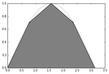
采用 trapezoidal 方法 和 simpson 方法 对这些采样点进行积分（函数积分为 2）：

result_s = trapz(y_s, x_s)
result_s_s = simps(y_s, x_s)
result = trapz(y, x)
print "Trapezoidal Integration over 5 points : {:.3f}".format(result_s)
print "Simpson Integration over 5 points : {:.3f}".format(result_s_s)
print "Trapezoidal Integration over 100 points : {:.3f}".format(result)

Trapezoidal Integration over 5 points : 1.896
Simpson Integration over 5 points : 2.005
Trapezoidal Integration over 100 points : 2.000

使用 ufunc 进行积分

Numpy 中有很多 ufunc 对象：

type(np.add)

numpy.ufunc

np.info(np.add.accumulate)

accumulate(array, axis=0, dtype=None, out=None)

Accumulate the result of applying the operator to all elements.

For a one-dimensional array, accumulate produces results equivalent to::

  r = np.empty(len(A))
  t = op.identity        # op = the ufunc being applied to A's  elements
  for i in range(len(A)):
      t = op(t, A[i])
      r[i] = t
  return r

For example, add.accumulate() is equivalent to np.cumsum().

For a multi-dimensional array, accumulate is applied along only one
axis (axis zero by default; see Examples below) so repeated use is
necessary if one wants to accumulate over multiple axes.

Parameters
----------
array : array_like
    The array to act on.
axis : int, optional
    The axis along which to apply the accumulation; default is zero.
dtype : data-type code, optional
    The data-type used to represent the intermediate results. Defaults
    to the data-type of the output array if such is provided, or the
    the data-type of the input array if no output array is provided.
out : ndarray, optional
    A location into which the result is stored. If not provided a
    freshly-allocated array is returned.

Returns
-------
r : ndarray
    The accumulated values. If out was supplied, r is a reference to
    out.

Examples
--------
1-D array examples:

>>> np.add.accumulate([2, 3, 5])
array([ 2,  5, 10])
>>> np.multiply.accumulate([2, 3, 5])
array([ 2,  6, 30])

2-D array examples:

>>> I = np.eye(2)
>>> I
array([[ 1.,  0.],
       [ 0.,  1.]])

Accumulate along axis 0 (rows), down columns:

>>> np.add.accumulate(I, 0)
array([[ 1.,  0.],
       [ 1.,  1.]])
>>> np.add.accumulate(I) # no axis specified = axis zero
array([[ 1.,  0.],
       [ 1.,  1.]])

Accumulate along axis 1 (columns), through rows:

>>> np.add.accumulate(I, 1)
array([[ 1.,  1.],
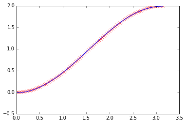
       [ 0.,  1.]])

np.add.accumulate 相当于 cumsum ：

result_np = np.add.accumulate(y) * (x[1] - x[0]) - (x[1] - x[0]) / 2

p = plt.plot(x, - np.cos(x) + np.cos(0), 'rx')
p = plt.plot(x, result_np)

​

​

速度比较

计算积分：$$\int_0^x sin \theta d\theta$$

import sympy
from sympy.abc import x, theta
sympy_x = x

x = np.linspace(0, 20 * np.pi, 1e+4)
y = np.sin(x)
sympy_y = vectorize(lambda x: sympy.integrate(sympy.sin(theta), (theta, 0, x)))

numpy 方法：

%timeit np.add.accumulate(y) * (x[1] - x[0])
y0 = np.add.accumulate(y) * (x[1] - x[0])
print y0[-1] 

The slowest run took 4.32 times longer than the fastest. This could mean that an intermediate result is being cached 
10000 loops, best of 3: 56.2 µs per loop
-2.34138044756e-17

quad 方法：

%timeit quad(np.sin, 0, 20 * np.pi)
y2 = quad(np.sin, 0, 20 * np.pi, full_output=True)
print "result = ", y2[0]
print "number of evaluations", y2[-1]['neval']

10000 loops, best of 3: 40.5 µs per loop
result =  3.43781337153e-15
number of evaluations 21

trapz 方法：

%timeit trapz(y, x)
y1 = trapz(y, x)
print y1

10000 loops, best of 3: 105 µs per loop
-4.4408920985e-16

simps 方法：

%timeit simps(y, x)
y3 = simps(y, x)
print y3

1000 loops, best of 3: 801 µs per loop
3.28428554968e-16

sympy 积分方法：

%timeit sympy_y(20 * np.pi)
y4 = sympy_y(20 * np.pi)
print y4

100 loops, best of 3: 6.86 ms per loop
0